Assignment 3

Goals and Background
The purpose and goals of this assignment are to investigate foreclosures in Dane County while using z-scores, probability, and the add field tool. Furthermore,  the experience acquired from this assignment in beneficial in helping to relate the calculated information (Z-Scores and Probability) to a situation for pattern analysis.

Key Terms

Z-Score: A Z-Score, also known as a standard score,  is a number that indicates how many standard deviations an element is from the mean and can be placed on a normal distribution.  Fig. 1 is the forumla for the Z score, where Zi: Z -score, Xi: number of observations minus the mean, divided by the standard deviation.

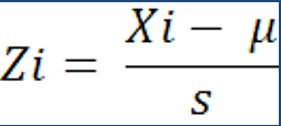
Figure 1: Z-Score Formula

Probability: Probability is the likelihood, by percent, that a numeric valued event will occur. The probability is derived from the z-score, then finding the Z-Score on a probability chart (Fig. 2). 

Probability Chart of Z-Scores

The Situation

      You have been hired by an independent research consortium to study the geography of foreclosures in a Dane County, Wisconsin.  County officials are worried about the increase in foreclosures from 2011 to 2012.  As an independent researcher you have been given the addresses of all foreclosures in Dane County for 2011 and 2012 and they have been geocoded and then added to the Census Tracts for Dane County.    While you realize that you cannot determine the reasons for foreclosures occurring, you do have the tools to analyze them spatially.  Specifically, you are interested to see how the patterns of these foreclosures have changed from one year to the next.  Explain what the patterns are and also provide some understanding as to the chance foreclosures will increase by 2013?  

After the calculation of the Z-Scores for the three tracts location in Dane County, a second question was given:

 If these patterns for 2012 hold next year in Dane County, based on this Data what number of foreclosures for all of Dane County will be exceeded 70% of the time?  Exceeded only 20% of the time?

Methods

First, a map was to be created displaying the change between 2011 and 2012 in foreclosures in Dane County, Wisconsin using ArcMap (Fig. 4).  A field was added to the attribute table, followed by using the field calculator to subtract the 2012 foreclosure value from the 2011 value.  The results offered a standard deviation classification and the ability to look at the differences between 2012 and 2011 regarding foreclosures in Dane County.

Next, the the instructions were to calculate the Z-Score for 3 specific tracts within Dane County (Fig. 3). Arcmap was then used to get the mean and standard deviation for both years of data.  The values for each three specific tracts from both years was plugged into Microsoft Excel, which was eventually used to calculate the the six Z-Scores using Excel ( Fig. 7).

Figure 3: Specific Dane County Tracts: 122.01, 114.01, & 31

Results

While examining Fig. 4, you can see the areas which have had a increase in foreclosures shown by the darker brown color on the outside of the map.  The areas with the green colors closer to the center of the county have seen a decrease in foreclosures since 2011.  It appears that areas outside of the central capital area in the center of the county are the areas that have faced higher foreclosure rates.  

Fig. 5 is a map showing the foreclosure value for 2011 accompanied with a standard deviation classification in the legend.  The standard deviation is needed to calculate the Z-Score for each of the three specific tracts.  Tract 114.01 has a higher amount of foreclosures compared to the county average.  Tract 122.01 has a lower number of foreclosures compared to the county average.  Tract 31 has a higher amount of foreclosures compared to the county average.  When comparing the results of Fig. 5 with the results of Fig. 4, it's notable that Tract 31 (in Fig. 5) has a higher than average amount of foreclosures, but in Fig. 4 there's a reduction in foreclosure numbers.  Similarly, the same thing appears in

Figure 5: 2011 Foreclosures

Fig. 6 is a map showing the foreclosure value for the year of 2012 with a standard deviation classification in the legend.  The results don't vary a lot between the three tracts; however, tract 31 did see a fair decrease from 2011 to 2012.

Figure 6: 2012 Foreclosures

Figure 7: Calculated Z-Scores of  three specific tracts from 2011 and 2012

Lastly, the second question that needs to be answered: 

If these patterns for 2012 hold next year in Dane County, based on this Data what number of foreclosures for all of Dane County will be exceeded 70% of the time?  Exceeded only 20% of the time?  

Foreclosures that had a Z-Score greater than -.52 will be exceeded 70% of the time.  This means that 70% of the time the foreclosures for a tract will exceed approximately 7.  

Foreclosures with a Z-Score greater than .84 will be exceeded only 20% of the time  This means that 20% of the time the foreclosures for a tract will exceed approximately 20.

Conclusion

There is a clear pattern of higher foreclosures on the outside of the county, surrounding the capital area of Dane County.  There isn't sufficient information to do a full analysis why the pattern is this way; however, there were some things uncovered that were significant. Around this time, the economy was recovering from a recession, and people who moved to the outskirts of Madison didn't anticipate problems such as a market crash.  In turn, this led to  rural areas outside of an urban area having a higher chance of having foreclosures as well as larger tracts because of the more expensive mortgages that come with suburban properties.  In order to find solution(s) for the high amount of foreclosures during this period, an investigation would have to be done to see how easy loans were given to these potential homeowners.  If the loans were given too easily, maybe the solution would be to make it harder to get loans for certain people.

Assignment 2 Geography 370

Goals and Background

The goal of the following assignment is to become familiar with a variety of statistical methods including Range, Mean, Median, Mode, Kurtosis, Skewness, and Standard Deviation. Furthermore, we will familiarize ourself with more programs such as MS Excel and ESRI Arc Map to help compute data we were given.

Definitions

Range

Range is the difference between the the largest value and the smallest value in a set of data. Example) say you had a data set of 1,3,5,7.  The range would be 7-1, which is 6.

Mean

Mean is average of all the numbers in a given data set. The mean is calculated by adding all of the numbers together and dividing the total by the total numbers of values in the data set. Example) 1,3,5,7.  1+3+5+7= 16.  16/4=4.  The mean is 4 in this data set.

Median

Median is the number which falls in the middle of a data set when put in order from smallest to largest. Example) 1,2,3,4,5.  3 is your median in this case.  If your data set has an even number of observations, you simply take the middle two values, add them together, and divide by 2.  Example) 1,2,3,4.  2+3=5.

5/2 =2.5.  2.5 would be the median in this case.  

Mode

Mode is the number which occurs most often in a data set. Example)  1,2,3,3,3,4,4,5,6.   In his case, 3 is the mode.  *Note* If there are two numbers that occur at the same frequency, then there can be two modes.

Skewness

Skewness describes the balance of the histogram compared to a normal distribution. There are 3 types of skewness: positive, no skew, and negative.  Positive skew is when the outliers in a data set are on the positive, or right side  of the mean (Fig.1). Negative skew is when the outliers in the data set are on the left side of the mean (Fig.1).  No skew means there is an even distribution of the data and the graph looks like a bell-shaped curve. 

Figure 1: Images containing postive and negative skewness http://study.com/academy/lesson/skewness-in-statistics-definition-formula-example.html

Kurtosis describes the shape of the histogram whether its "steep," or "flat" o compared to the "normal distribution.There are 3 different ways to describe Kutosis: Leptokurtic, Mesokurtic, and Platykurtic.   Leptokurtic is a description of a very peaked or "steep" distribution. Mesokurtic is deemed to have a  "normal" distribution. Platykurtic is a short or a "flat" distribution. Additionally, Platykurtic is described as negative Kurtosis and Leptokurtic is positive Kurtosis. Figure 2 below is an example of the three types of Kurtosis. When analyzing Kurtosis calculations anything greater than 1 is Leptokurtic and below -1 is Platykurtic.

Figure 2: The forms of Kurtosis.  http://mvpprograms.com/help/mvpstats/distributions/SkewnessKurtosis

Standard Deviation

Standard Deviation is a statistical measurement which describes how spread out the numbers in a data set are from the mean. "1 Standard Deviation" from the mean is equal to 68.2% of the values in a data set. "2 Standard Deviations" from the mean is equal to 95.4% of the values in a data set.  "3 Standard Deviations" from the mean is equal to 99.7% of the values in a data set. 

Assignment Description - Part 1

We were given the following scenario by our professor:

Cycling is often seen as an individual sport, but it is actually more of a team sport.  You are looking to invest a large sum of money into a cycle team.  While having a superstar is nice and brings attention, having a better team overall will mean more money in your pocket.  In the last race in the TOUR de GEOGRAPHIA, the overall individual winner won $300,000, with only 25% going to the team owner, but the team that won, gained $400,000 in a variety of ways, with 35% going to the team owner.  

Using the incredible set of knowledge learned in your Quant Methods class at UWEC, you decide to put it to good use.  You have data (total time for entire race) for teams and individual racers over the last race held in Spain. To begin your investigation you are to analyze the race times of members from the team. Traditionally Team ASTANA has typically produced the race winner (meaning the rider that finishes first), but an up and coming group named Team TOBLER has been making waves on the cycling circuit.  

The questions that will be answered are as follows:

Should you invest in Team ASTANA or gamble on Team TOBLER?   Why did you pick one team over another?  What descriptive statistics do you think best help explain your answer?  Please explain your results using the statistics to support your answer **Please explain results in hours and mins. 

Methods

For this assignment I had to calculate the Range, Mean, Median, Mode, Kurtosis, Skewness, and Standard Deviation for the race times provided to me.The standard deviation was to be calculated by hand and shown on paper, as figures 3 and 4 provide the proof below.  The rest of the results could be calculated in MS Excel itself.

I first calculated the standard deviation of each team (Fig. 3-4) using the population standard deviation formula.  Figure 3 and 4 provide the work I did for both Team Tobler and Team Astana.  

 I then copied the provided data and imported it into Excel so I could sort the numbers in descending order.  After  that, I was able to calculate the Range, Mean, Median, Mode, Kurtosis, Skewness for each team using Excel and the results are shown below in table 1.

Figure 3: Calculating the Standard Deviation of Team Tobler

Figure 4: Calculating the Standard Deviation of Team Astana

Table 1 Results

Table 1

Discussion and Answer

It's hard to answer whether I'd invest in team Astana or gamble on Tobler.  Based on the results of the data set given, I would likely invest with team Astana because the mean is a very safe number.  However, this is the results of one race, and one race results isn't enough for me to make a solid decision on which team to invest money into.  
Some more reasons I would choose Team Astana over Team Tobler is that the total time (sum)  for Astana was equal to 569 hours and 10 minuets versus Tobler which had a total time of 571 hours and 21 minuets.  Team  Tobler had a lower standard deviation, meaning the team had fewer outliers and most the team finished around the same time.  In spite of the lower standard deviation, the majority of team Tobler finished behind team Astana. Team Astana had a higher standard deviation because of Racer K, who possibly had a bad day running, which in turn made Team Astanas standard deviation higher.  




Assignment Description - Part 2

For part 2 we are to calculate the mean center and weighted mean center for the population of Wisconsin by county for 2000 and 2015.  Before that, I will provide the important definitions for part 2 below.  

Mean Center

The mean center is the average location of points which have an X and a Y value and are plotted on a graph or Cartesian Plane.  

Weighted Mean Center

The weighted mean center is a set of points that is adjusted in order to influence a second value associated with each point.  The difference between this and mean center is that the points have weights or "frequencies" attached to them (Fig. 5)


Figure 5: Geographic Mean Centers of Wisconsin Population from 2000 and 2015.

Discussion and Conclusion

In the above map, you can see the mean center is centrally located in the state.  The mean center is calculated off of the center point of each county, which is why it is located in the center of the state. The weighted mean centers are still in central Wisconsin, but further south from the mean center.  That is because the weighted mean center takes the population of counties into account.  The more populated counties are all in the southern and southeast part of the state, specifically Milwaukee County and its' surrounding area.  You can see that the weighted mean center from 2015 is slightly west of the 2000 weighted mean center.   It appears that there has been a population shift from 2000 to 2015, possibly to get closer to other working centers such as La Crosse, or the Twin Cities in Minnesota.